1. Background of Particle Image Velocimetry

Particle Image Velocimetry (PIV) is a laser diagnostic method which has been developed in parallel with Laser Sheet Visualization (LSV) (CF 119). As with LSV, it is based on the collection of images of [GLOSS]Mie scattering[/GLOSS] of fine particles seeded in the flow. Processing of these particle images provides instantaneous data on two velocity components in a plane crossing the flow. Then, the mean and root-mean-square (rms) velocity fields can be easily deduced from statistical studies of the instantaneous measurements sequences.

In the last ten years, the PIV technique has shown rapid expansion thanks to developments of illumination sources (lasers) and image collection systems ([GLOSS]CCD Camera[/GLOSS]s), as well as specific image processing algorithms based on cross-correlation calculations accessible with increasing performance of computer speed and memory size [1, 2]. Nowadays, the use of this laser diagnostic has been enlarged to all applications of experimental fluid mechanics, notably in combustion. Several optical diagnostic commercial suppliers offer turn-key PIV systems. However, attention has to be paid to the results obtained form these turn-key system, especially in regard to dynamic measurements, spatial and temporal resolutions, and other possible experimental biases in complex flows such as turbulent flames.

Actual applications of PIV technique are focused on time resolved PIV for the description of temporal behaviour of turbulent flows, as well as on stereo-PIV for measurements of 3 velocity components in a plane, and holographic PIV for complete velocity measurements in a volume. PIV algorithms are also still being improved in order to increase spatial resolution, reduce measurement errors and optimise computer time consumption. Recent developments and applications of PIV are regularly presented during each successive “International Symposium of Particle Image Velocimetry” [3].

 

The application of PIV in industrial scale flame has been already demonstrated on a 1MW experimental boiler [4]. More details on its application at such industrial scale combustion facility is presented in CF278.

2. Principle of Particle Image Velocimetry

Particle Image Velocimetry can be considered as two successive steps: first the collection of particle images in the flame, and second their processing for the determination of velocity fields. These two steps can be done separately to minimize the duration of the experiment.

 

Image acquisition and digitisation

The experimental set-up of PIV is basically the same as LSV. It requires specific equipment (laser, CCD camera, etc) to be able to acquire couples of tomographic images separated by a short time delay. Figure 1 shows a scheme of the PIV setup on a laboratory flame.

The investigated flow – the flame in our case – is seeded with tracer particles. The latter must have a low density and be small enough to follow the flow in the whole of the turbulence spectral range. Aluminium oxides (Al₂O₃) and zirconium oxides (ZrO₂) particles are often chosen for combustion studies because of their ability to be still present in the flame. In practice, the seeding of the flow is done in the laboratory, thanks to a seeding machine with different concepts: fluidised bed, cyclonic seeder, rotary brush seeder, etc.

For PIV, the seeded flow is illuminated by a specific laser delivering couples of pulses, usually a double cavity [GLOSS]ND:YAG laser[/GLOSS]. The short duration of each laser pulse (~ 10 ns) ensures there are snapshots of the “frozen” flow. A set of spherical and cylindrical lenses are used to turn the circular laser beam into a laser sheet, which is the measurement plane of velocity fields by PIV. In the simplest configuration, the spherical lens controls the width of the laser sheet (usually less than 500 μm), whereas the cylindrical one induces the divergence of the laser beam, i.e. the height of the laser sheet. During laser pulse, particles crossing the laser sheet scatter the light. The Mie scattering signal is collected by a CCD camera set perpendicularly to the measurement plane (Figure 1). The two exposures of the particle field from the double pulsed laser are recorded on two separated frames thanks to a precise synchronicity between the laser and the CCD camera. The time delay δt between the two successive laser pulses is adjusted to the flow characteristics. It is a compromise between a large value, to have a noticeable displacement of particles in the whole field of view, and a small value to avoid loss of particles between the first and the second images, notably due to out-of-plane particle motion.

 

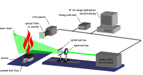
Figure 1. Diagram of the PIV setup on a laboratory flame

 

Image processing

This section presents the methodology of data processing performed on each couple of particle images to obtain an instantaneous velocity field.

 

Each image is divided into a grid of small areas (Figure 2), called the interrogation window (IW). Dimensions of IW are chosen to have a minimum of 10 particles (usual values are 32 x 32 pixel²). Then [GLOSS]cross-correlation[/GLOSS] (CC) between the first and the second image is calculated in each interrogation window, usually thanks to fast Fourier transforms (FFT).  The CC calculation result has a peak which position (δx_p ; δy_p) corresponds to the most probable displacement of the particles in the IW. Interpolation of the peak, usually by a Gaussian fit, gives sub-pixel values – i.e. non integer – of δx_p and δy_p to increase accuracy of the measurement, and then widen dynamic of the PIV technique [5]. The same calculation repeated on each IW gives a complete field of particle displacement.

 

Currently, most PIV algorithms offer also an iterative procedure of CC calculation where the IWs are shifted to catch up with the particle loss in the IW pattern during the δt delay and minimize algorithmic bias called “peak locking” [6]. In addition, the IW can be resized [7] or re-oriented [6] during the iterative procedure in order to improve the spatial resolution.

 

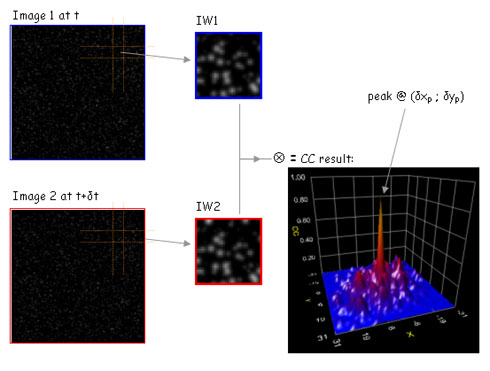
  Figure 2. Procedure of CC calculation of particle images

 

The next step of the data processing concerns the scaling of the pixel positions (x_p ; y_p) of the images and the calculated particle displacements (δx_p ; δy_p). This is performed by [GLOSS]magnification functions[/GLOSS] giving real (x_r ; y_r) positions and (δx_r ; δy_r) displacements in the laboratory frame of reference. These functions are determined by imaging a square grid pattern set in the plane of the laser sheet. In most configurations, magnification functions are found to be linear.

Then the flow velocity attributed to the corresponding real position (X_r ; Y_r) of the centre of each IW is obtained from the basic equation:

 

 

Some experimental biases, e.g. low particle density, out-of-plane particle motion, etc. may induce a poor quality of the CC calculation and resulting incorrect values in the instantaneous velocity field. Such spurious vectors can be eliminated by appropriate filtering. There are two types of filters. Global filters are defined from minimum and maximum values of velocity components fixed a priori, below or above which the velocity result is not validated. Local filters are based on local continuity of the flow. Each PIV result is compared with its neighbours, and is eliminated if it is considered as too far from them [8]. There is not one ideal filtering method suitable for all experimental configurations. As some filter parameters are subjective, they have to be changed and tested on a few raw instantaneous velocity fields in order to be adapted to each situation. At the end of the filtering step, spurious measurements are interpolated to provide the complete instantaneous velocity field.

 

Limits of dynamic range of PIV measurements come mainly from CC calculation. Measurement of 0.1 pixel is commonly considered as the minimum reliable value for particle displacement, whereas the maximum calculable displacement is roughly defined as one third of the IW size. Accuracy of each measurement is tricky to quantify as it depends of the considered experiment. In the most favourable conditions, it can be estimated as less than 0.1 pixel, but can increase notably in the case of strong gradient in the IW [7]. Conversion of these limits into absolute values of velocity thanks to the delay time dt and the magnification functions gives an estimation of the maximum dynamic range for each experiment.

 

Characterization of turbulent flames requires the performance of a statistical study of PIV measurements. This is done in a post-processing step by calculating mean and root-mean-square (rms) velocity fields from a group of instantaneous ones. Several other spatial derivatives, e.g. vorticity, divergence, and gradient can also be deduced from instantaneous velocity fields obtained by PIV to enhance further aerodynamic characterization of the flow.

 

3. Example on a laboratory Bluff-Body gas burner

CH4

air

Bluff-Body

air

Figure 3. Picture of the bluff-body burner flame

This section presents some results of the application of PIV to a laboratory [GLOSS]bluff-body[/GLOSS] gas burner mainly obtained by Arnaud Susset during his PhD Thesis carried out within the framework of a collaboration between the Gaz de France – LCD (UPR 9028 CNRS – ENSMA) and CORIA (UMR 6614 CNRS, Université et INSA de Rouen) laboratories [9].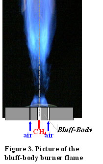

 

Figure 3 shows a typical flame generated by the 20 kW axisymetric bluff-body burner. Methane is injected through the centre of the bluff-body at a velocity of 21 m.s^-1. Air is supplied as an annular jet surrounding the bluff-body at a velocity of 7.5 m.s^-1. The flow field generated by the burner is characterized by the interaction of the central jet of methane and the coaxial air jet in the [GLOSS]internal recirculation zone[/GLOSS] (IRZ) generated by the wake of the bluff-body, conducive to flame stabilization. Downstream of this IRZ, one can observe an axial extinction region and a secondary reactive region which develops into a jet-like flame.

The PIV setup on this burner consists of rotary brush seeders set directly on the methane supply system and in by-pass on the air supply system. Added to the convergent and cylindrical lenses, another convergent lens with a large diameter is used to control the divergence of the laser sheet. A large CCD camera (1280 x 1024 pixel²) is used, as it favours the spatial resolution. Its frame transfer signal is used as the master base for the temporal synchronization of the double cavity Nd-YAG laser (10 ns – 400 mJ/pulse) and other electronic devices.

Instantaneous velocity fields have been measured from couples of particles images, for example the one shown figure 4. Total processing time is in the order of 5 seconds for each instantaneous field. Figure 5 presents the mean velocity field obtained from the ensemble average of 1000 instantaneous fields.

image #1

image #2

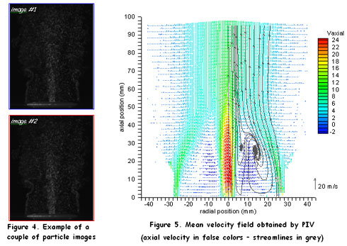
One clearly observes the presence of a toric IRZ at the exit of the burner, generated by a methane centrifugal vortex and an air centripetal vortex. This leads the mixing of methane and air in region with large resident time where the flame stabilizes. Moreover, study of instantaneous velocity fields obtained by PIV has allowed us to describe the temporal evolution of the flame during the intermittent phenomenon of [GLOSS]vortex shedding[/GLOSS] from the IRZ to the jet-like flame [9]. This illustrates the ability of the PIV technique to give new insights in the aerodynamic study of flame.

Sources

[1] R.J. Adrian, “Particle-imaging techniques for experimental fluid mechanics”, Annu. Rev. Fluid Mech., vol. 23, pp. 261-304, 1991.

[2] C.E. Willert, M. Gharib, “Digital particle image velocimetry”, Experiments in Fluids, vol. 10, pp. 81-193, 1991.

[3] http://piv03.snu.ac.kr

[4] D. Honoré, S. Maurel, A. Quinqueneau, “Particle Image Velocimetry in a semi-industrial 1 MW boiler”, Proceedings of the 4^th International Symposium on Particle Image Velocimetry, Göttingen, Germany, Sept. 11-19, 2001.

[5] J. Westerweel, D. Dabiri, M. Gharib, ” The effect of a discrete window offset on the accuracy of cross-correlation analysis of digital PIV recordings”, Experiments in Fluids, vol. 23, pp. 20-28, 1997.

[6] B. Lecordier, D. Demare, L.M.J. Vervisch, J. Réveillon, M. Trinité, ” Estimation of the accuracy of PIV treatments for turbulent flow studies by direct numerical simulation of multi-phase flow”, Meas. Sci. technol., vol. 12, pp. 1382-1391, 2001.

[7] A. Susset, J.M. Most, D. Honoré, “A novel architecture of super-resolution PIV algorithm for the improvement of large velocity gradient resolution”, Proceedings of the 5^th International Workshop on PIV, Busan (Korea), Sept. 22-24, 2003.

[8] J. Westerweel, “Efficient detection of spurious vectors in particle image velocimetry data”, Experiments in Fluids, vol. 16, pp. 236-247, 1994.

 [9] A. Susset, “Développement de traitements d’images pour l’étude de la stabilisation de flames turbulentes non-prémélangées générées par des brûleurs industriels modèles”, PhD Thesis, Université de Poitiers, 2002.