What is an Artifical Neural Network (ANN)?

SIGN IN

What is an Artifical Neural Network (ANN)?
Date posted: 31st May 2003
Share this post
- Post Author
  
  espadmin

1. Background

The past fifteen years or so have seen an increasing use of [GLOSS]Artificial neural network[/GLOSS]s (ANNs) to model or represent a large class of “real” problems and systems which are very difficult to analyse by conventional methods. These systems, including some in the field of combustion, are frequently characterised by the following features:-

§ It is not always possible to develop a mathematical model for the system or problem that adequately represents the actual physical processes.

§ The solution methodology employed by a “human expert” is often based on a discrete rule-based reasoning framework. Attempts to generalise these rules in a conventional expert system can often be difficult.

§ The complexity and size of the problem is such that “hard and fast rules” cannot easily be applied and, moreover, the computational requirements of conventional models can be excessive.

There are many different types of ANN, see for example, Jain et al. (1996). However, typically an ANN is made up of a large number of interconnected processing elements linked together by connections. The essential structure of the network is therefore similar to that of a biological brain in which a series of neurons are connected by synapses. An ANN can be characterised by a massively distributed and parallel computing paradigm, in which “learning” of the process replaces a priori program and model development. The learning phase can be understood as the process of updating the network structure and [GLOSS]connection weights[/GLOSS] in response to a set of [GLOSS]training data[/GLOSS] obtained from experimental measurements or, less often, from a rigorous mathematical model of the process. The overall behaviour and functionality of an ANN is determined by the network architecture, the individual neuron characteristics, the learning or training strategy, and the quality of the training data. Once trained the network has a relatively modest computing requirement.

It must be emphasised that an ANN is a relatively simple method of representing complex relationships between parameters for which corresponding data is already available. No new knowledge is generated by an ANN, but the approach is often easier and more effective than conventional curve fitting techniques, or computer models based on the underlying physical and chemical processes. In particular, an ANN offers the capability of simulating and even controlling a combustion process in real time, as well as being a powerful tool for the classification of complex data sets.

2. The Feed-Forward Multilayer Perceptron Network

The Feed-Forward Multilayer Perceptron Network (FFMLP), as shown in Figure 1(a), is the most popular [GLOSS]supervised learning[/GLOSS] network and has found application across many disciplines, including combustion, see Wilcox et al. (2002). It is particularly suited for use in tasks involving prediction and classification of complex data. A FFMLP network is typically organised in a series of layers made up of a number of interconnected neurons each of which contain a [GLOSS]transfer function[/GLOSS], f (Figure 1(b)). Input data are first presented to the network via the [GLOSS]input Layer[/GLOSS], which then communicates this data via a system of weighted connections to one or more, [GLOSS]hidden Layer[/GLOSS]s where the actual neuron processing is carried out. The response of the hidden layers is then transferred to an [GLOSS]output layer[/GLOSS] where the network outputs are computed. During the training phase these outputs are compared with known “target” values for the process. The resultant errors arising from the difference between the predicted and known values are back-propagated through the network and used to update the weights of the connections. The process is successively repeated until the errors fall within pre-specified limits. At this stage the network training is said to be complete. However, it should be appreciated that training is not necessarily a “once-off” procedure since the network can “learn” and be updated on-line if the system or process changes.

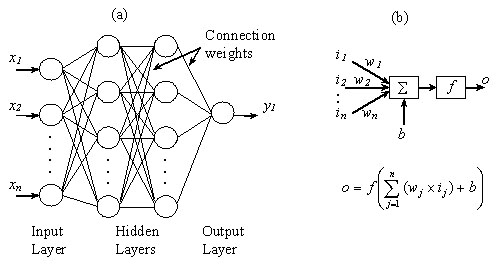
Figure 1: (a) Typical ANN Architecture and (b) Computational Model of a Single Neuron.

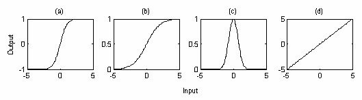
Figure 2: Neuron Transfer Functions. (a) ‘Tansig’ (b) ‘Logsig’ (c) ‘RBF’ and (d) ‘Purelin’.

The three most widely used transfer functions for the hidden neurons are (a) the tanh-sigmoid (tansig), (b) log-sigmoid (logsig) and (c) the radial basis function (RBF), whilst a commonly used transfer function for the output neurons is a linear function (purelin) (Figure 2). As a result of the use of these non-linear transfer functions in the hidden neurons, a FFMLP network can successfully represent highly complex input-output relationships so that it can often be employed as a “black box” model of a system or process. A simple example of the use of a FFMLP is presented in CF237 “How do I use a neural network to predict the calorific value of a solid fuel”.

3. Training an ANN

The successful implementation of an ANN should take into account the following features, which can affect the performance of the trained network.

Data Pre-Processing

Neural network training can be made more efficient if certain pre-processing steps are performed on the network inputs and targets to prevent individual parameters dominating the response. One way of doing this is to scale the inputs and targets so that they fall in the range [-1, 1]. Another useful approach is to normalize the values so that they have a zero mean and unit standard deviation.

The Number of Hidden Neurons

The response of a neural network is sensitive to the number of neurons in the hidden layer(s). The use of too few neurons can lead to under fitting of the training data whilst too many neurons can contribute to over fitting. In this latter case all the training values are closely represented, but the relationships predicted by the network can oscillate wildly between these points. Consequently large errors can occur during subsequent prediction of previously unseen conditions. Unfortunately, there is still no single reliable method, apart from trial and error, to determine the optimal number of hidden neurons for a particular application.

Number of Output Neurons

The number of output neurons is problem specific, in that it depends on how many dependent variables are modelled. In some cases each dependent variable is modelled using a separate network since this allows more efficient training of smaller networks and hence can improve [GLOSS]generalisation[/GLOSS] of the network.

Use of Feed-back Connections (Recurrent Networks)

With time varying data a FFMLP network can be made recurrent by the addition of feed-back connections, (with appropriate time delays), from either the outputs of the hidden layers to the inputs (internal feed-back connections) or from the output neurons to the input layer (global feed-back connections). These feed-back paths allow the network to both learn and store the time-varying patterns in the training data and consequently this type of network is particularly useful for modelling time-dependent or dynamic systems.

4. Generalisation of the Network

Following successful training, the outputs of the network should adequately “match” the target values corresponding to the given inputs in the training data set. Usually, however, the purpose of using a neural network is to predict or control the behaviour of a system for a range of previously unseen input data, i.e., the network should be capable of generalisation. Neural networks do not automatically generalise, and care should be exercised in interpreting network predictions. In this context it is important that continuous functional relationships (albeit highly complex, approximate and unspecified) exist between the system inputs and outputs. Moreover, the training data should be sufficiently large to be representative of the whole problem domain since neural networks can be usually only used reliably to interpolate within the range of the training conditions. Therefore ANN predictions are often subject to significant errors if the network is applied to the region of a system where the initial training data are “sparse”. Furthermore the use of an ANN to extrapolate the behaviour of the system to conditions which lie outside the range of the training data is notoriously unreliable. Hence it is important to have sufficient, and suitably distributed, training data to obtain satisfactory predictions and to avoid the need for extrapolation.

Sources

Jain, A.K., Mao, J.C. and Mohiuddin, K.M. (1996) Artificial Neural Networks: A Tutorial. Computer, 29(3): 31-44.

Wilcox, S.J., Ward, J., Tan, C.K., Tan, O.H. and Payne, R. (2002) The Application of Neural Networks in a Range of Combustion Systems. Proc. 6^th European Conference on Industrial Furnaces and Boilers, Estoril, Portugal, 4: 203-214.