1. Background

Laser Sheet Visualisation ([GLOSS]LSV[/GLOSS]) of fluid streams seeded with micron-size particles may be used to obtain images of the mixing field between fuel and comburent in a flame (CF119, 123).

The same data may also be analysed to yield qualitative or semi-quantitative information on mixing parameters using the approach outlined in this Combustion File (CF).

A further Combustion File (CF134) deals with the specific determination of [GLOSS]unmixedness[/GLOSS] from the same data.

2. Principle of Mie Scattering

Application of the [GLOSS]Mie scattering[/GLOSS] technique to study mixing is described in CF119 and in more detail in sources [2 to 4].

Under ideal conditions, the instantaneous light scattering intensity (I) is directly proportional to the number of particles in the control volume. Thus:

I = krZ                   (1)

where:

Z is a value equivalent to the mixture fraction of the seeded fluid

r is the fluid density in the control volume (kg/m³)

k is a constant of proportionality

The mixture fraction is usually normalised to its initial value in the seeded flow, defined as unity. Thus:

Z = (I/I₀) x (r/r₀)                            (2)

where:

I₀ is the value of scattered light intensity from the undiluted fluid, typically determined by a measurement in the [GLOSS]potential core[/GLOSS] of the jet of seeded fluid of density r₀

The value of Z defined in this way is analogous to (but numerically different from) the aerodynamic mixing factor m_a that can be determined from species concentration measurements in a flame (CF 116).

It can be further noted from equations (1) and (2) that for experiments in non-reacting flows involving two fluids of identical density, the calibrated Mie scattering signal (I/I₀) is strictly equivalent to the Z.

3. Analysis of Laser Flame Visualisation Data

In order to undertake quantitative analysis, a large number of images (several hundreds) from a Laser Sheet Visualisation [GLOSS]CCD Camera[/GLOSS] must be recorded (eg on videotape) and then transferred to the hard disk of a computer [2].

Each of these images corresponds to a single laser pulse illumination that provides a frozen view of the seeded stream.

The image sequence may then be analysed with automatic image-analysis procedures such as those developed at the IFRF.

In order to yield a quantitative number density, the analysis software must also calibrate the instantaneous images and correct them for non-homogeneous illumination and optical path attenuation (CF119).

The images are scaled so that the unmixed seeded fluid corresponds to a mixture fraction of 1, while the minimum signal intensity, found in the un-seeded flow, corresponds to a mixture fraction of zero.

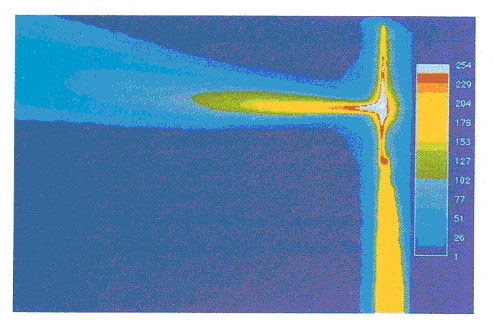
Figure 1: Calibrated particle number density

The pseudo-colour scale ranges from 0 to 255 (normalized
number density I/I₀ = 1 in jet potential core)

In single fluid or constant density non-combusting flows, the mass fraction is calculated from the calibrated number density and the air and seeded (fuel) stream molecular weights.

In combusting flows, calculation of the mass fraction requires knowledge of the instantaneous temperature because the particle number-density signal is proportional to the product of the mass fraction and the fluid density (equation 2).

It is common [3] to apply the assumption of fast and irreversible chemistry and unit [GLOSS]Lewis number[/GLOSS]in order to provide a simple relationship between the mixture fraction, and the density. This in turn allows the calculation of the flow temperature (T), and mixture fraction from the calibrated number density (I/Io).

This assumption is valid in large-scale flames (high [GLOSS]Reynolds Number[/GLOSS]and [GLOSS]Damkholer number[/GLOSS]) in which mixing is controlled by turbulent diffusion. These relationships are given in Figure 2 for natural gas/air combustion.

In Figure 2, F_st is the stoichiometric mixture fraction, T_ad the adiabatic flame temperature, and I/I₀ is the normalized light intensity from the seeded natural gas stream potential core.

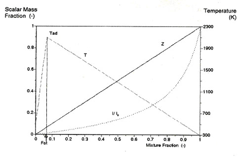
Figure 2: Instantaneous relationships for infinitely fast and irreversible reactions in turbulent diffusion flames

Thus, the assumption of a monotonic relation between the calibrated particle number density and the mixture fraction enables the instantaneous temperature and mixture fraction to be derived. The analysis procedure then calculates the mean and fluctuating temperature and conserved scalar fields.

For rapid evaluation and appreciation of the data, it is useful to display the results as false colour images.  An example of such images produced by the IFRF software is shown in Figure 3, which shows the progress of mixing between the natural gas and the combustion air within the flame.

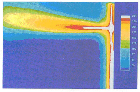
Figure 3: Average mixture fraction field

This mixing map is equivalent to (but numerically distinct from) the [GLOSS]aerodynamic mixing factor[/GLOSS] m_a (CF 115, CF116) that may be determined from species concentration measurements.

Compared to detailed point by point in-flame measurements with a sampling probe, the Laser Sheet approach is fast and simple to implement. It allows the characterisation of several jet mixing properties such as the intermittency, the unmixedness, jet boundaries, and the jet expansion angle [4].

When the Laser Sheet Visualisation is also used to determine unmixedness (CF134), the data may also be processed to yield the maximum value of the [GLOSS]degree of oxidation[/GLOSS] (CF118).

It must be noted that, unlike species concentration measurements, the present mixing based LSV approach is unable to account for lags in the combustion reactions caused by the reaction kinetics or the reaction equilibria (CF31).

4. Errors in the quantitative output

Random errors arise in the LSV data as a result of seeding fluctuations and noise on the output of the CCD camera.

The significance of a random error on a time averaged parameter decreases as the square root of the number of samples increases.

At the IFRF, a sequence of 350 LSV images was found to reduce the random error in the calibrated particle number density to 0.1% of full scale.

Under these conditions, and also taking account of systematic errors due to optical attenuation, non-uniform illumination and non-linearities in the camera response, a total error of 5% of the dynamic range results.

5. How do I take things forward?

The relationships and explanations given above may be used as a starting point to develop in-house hardware and software for Laser Sheet Visualisation analysis.

Alternatively, they may be used to help inform purchasing decisions regarding the acquisition or use of proprietary systems, including that developed by the IFRF.

IFRF Members may also seek further detailed advice and guidance from the IFRF Research Station.

Sources

[1]IFRF Doc C76/y/3/2

[2] Dugué, I., Mbiock. A. and Weber, R (1994). Mixing characterisation in semi-industrial natural gas flames using planar Mie scattering visualization. 7th Int. Symp. on Applications of Laser Techniques to Fluid  Mechanics, Lisbon. 4

[3]Stepowski, D. (1992) Laser measurement of scalars in turbulent diffusion flames Prog. Energy Comb. Sci., vol 18, pp. 463-491.

[4] J Dugué, H Horsman, A Mbiock & R Weber. Flow Visualization and Mixing Characterization in Industrial Natural Gas Flames. 1995-International Gas Research Conference, Vol II, V. Industrial Utilization, pp. 2122-2131; France, Cannes, 6-9 November 1995.