1. Background

The concept of [GLOSS]calorific value[/GLOSS] was introduced in combustion file CF21. Both the net calorific value ([GLOSS]lower calorific value[/GLOSS]) and the [GLOSS]gross calorific value[/GLOSS], ([GLOSS]higher heating value[/GLOSS]) of solid fuels can be calculated in an approximate manner from a knowledge of the [GLOSS]ultimate analysis[/GLOSS] of the fuel by using empirical formulae, see for examples CF225 and CF105. These formulae are derived using [GLOSS]multiple linear regression[/GLOSS] (MLR) analysis, which assumes linear relationships between the independent variables (measurements of the ultimate analysis) and the dependent variable (i.e., the calorific value).

However, an [GLOSS]artificial neural network[/GLOSS] (ANN) technique, with its inherent ability to represent complex, non-linear data, can be used as an alternative to predict the calorific value. The basic features of a neural network are described in CF46,”What is an artificial neural network?” This current file is intended to provide a simple demonstration of how such a network can be employed successfully in a combustion application. The approach described in this file is based on the use of a proprietary neural network, Matlab^® Neural Network Toolbox, in order to illustrate the generic ANN approach and its capabilities.

2. The Database of Fuel Properties

In order to train a neural network, a data set giving calorific value and the ultimate analysis of a range of fuels is required. For the purposes of the test example shown below, a collection of fuel properties for a variety of coals, biomass and waste materials was extracted from the Phyllis database [1] and used as data to train the neural network. As an alternative, other data may be found in the IFRF Handbook by searching against keywords such as ‘data’ or ‘fuels’.

In order to assess the ability of the trained ANN to predict unseen conditions a separate set of test data were obtained from Jenkins and Ebeling, [2]. The ultimate analysis of the fuels including carbon (C), hydrogen (H), oxygen (O), nitrogen (N) and sulphur (S) contents (expressed as a percentage by mass) were used as inputs to the network and the corresponding higher heating values (HHV) as outputs. A total of 259 samples were employed for training with 45 values for testing. Table 1 indicates the numerical ranges of the data.

Table 1: Fuel compositions (% by mass) and heating values

Data Preprocessing

Prior to training the neural network, the data should be normalised to give a zero mean and unit standard deviation. 

3. Neural Network Training

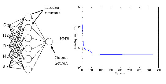
The Matlab^® Neural Network Toolbox [3] was used to configure a standard feed-forward multilayer perceptron network (FFMLP) with 6 tanh-sigmoid [GLOSS]hidden neurons[/GLOSS] and 1 linear output neuron to model the data (Figure 1a). The network was trained by means of a [GLOSS]Bayesian regularization[/GLOSS] technique to minimise any effects of over-fitting of the data, and during training the ANN converged to a sum-square error of 4.56 in 371 [GLOSS]epochs[/GLOSS] (Figure 1b).

Figure 1: (a) network architecture (b) training history (sum-square-error)

4. Results

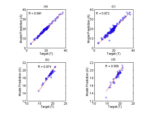
The trained network was used to predict the test data set and as a comparison, the network performance was compared with Boie’s equation found in CF105. The ability of the network and the equation to fit both the training and test data is illustrated in Figure 2. It can be seen that the neural network model slightly outperforms Boie’s equation over the very wide range of solid fuels examined. Correlation coefficients (R-values) of 0.991 and 0.974 were achieved for the training and test data respectively with the ANN as compared with 0.974 and 0.956 when Boie’s method was used. Consequently an artificial neural network can provide a suitable alternative method for predicting the calorific value of both coals and biomass materials from a knowledge of the fuel composition.

Figure 2: Scatter plots of predicted versus actual HHV. (a) neural network (training data), (b) Boie’s equation (training data), (c) neural network (test data) and (d) Boie’s equation (test data).

[1] Phyllis – the composition of biomass and waste. http://www.ecn.nl/phyllis/.

[2] Jenkins, B.M. and Ebeling, J.M. (1985). Correlation of Physical and Chemical Properties of Terrestrial Biomass with Conversion. Symposium on Energy from Biomass and Wastes, Inst. Of Gas Technology, Chicago, IL, USA, pages 371-403.

[3] Demuth, H. and Beale, M. (2001). Neural Network Toolbox User’s Guide (version 4). The MathWorks, Inc.