1. Background

In the past, to increase their level of understanding of industrial
combustion systems operation, and to carry out design optimisation or combustion
improvements, engineers have had to resort to sometimes to full-scale
experimentation or to so-called semi-industrial scale experimentation carried
out at laboratories such as that at the IFRF.

Prohibitive time constraints and cost issues led engineers to develop
alternative options such as proper modelling techniques, both physical and
mathematical, in order to obtain a valid representation of the phenomena
occurring in their systems.

The relatively “young” numerical modelling tool, also referred to as [GLOSS]Computational Fluid Dynamics[/GLOSS] (CFD), boosted by the progress leap in computing
systems development and researchers ingenuity, is increasingly supporting the
energy intensive sector’s of industry in the areas of: feasibility and design
assessment; process and emissions control and improvements; “what if”
developments… etc., etc..

CFD describes fluid flow systems. Those are governed by the laws of conservation
of mass, momentum, energy, chemical concentrations, and other physically
meaningful quantities expressed with models (e.g. [GLOSS]Turbulence[/GLOSS], [GLOSS]combustion[/GLOSS], radiation,…), together with a set of constitutive relations for the fluid.

All flows of industrial relevance, such as combusting systems, are taking place
under a turbulent regime.

This general Combustion File introduces a light background on turbulence
modelling and highlights the maze of existing possibilities offered to each
modeller, introducing three specific procedures or sub-models, which are
detailed in separate CFs – see Related Combustion Files.

2. What is turbulence?

One of the most famous non-dimensional criteria used by engineers since the turn
of the last century is the [GLOSS]Reynolds Number[/GLOSS] (Re). We all know that, above a
critical value of the Reynolds Number, the flow regime in a system is classified
as TURBULENT.

However, can TURBULENCE be clearly defined? Well, not really. A chaotic and
random state of motion develops, in which the velocity and pressure change
continuously with time within substantial regions of the flow. The motion
becomes intrinsically unsteady even with stationary imposed operating
conditions, otherwise referred to as boundary conditions. All other flow
properties start to behave likewise, so that the overall flow characteristics
are seen to be:

• Unsteady and highly irregular in space and time.
• Strongly diffusive, causing rapid mixing and increased rates of momentum
  transfer.
• Dissipative: the kinetic energy of turbulence is converted into heat via work
  done against viscous stresses.

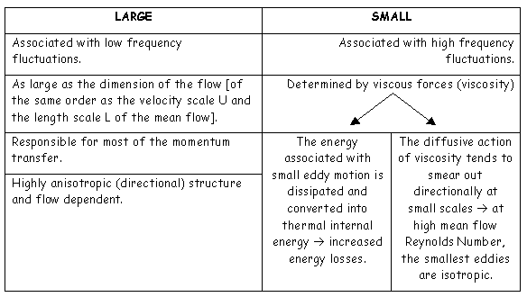
Turbulent fluctuations always have a 3D spatial character and turbulent flow
visualisation reveals the formation of rotational flow structures, so-called [GLOSS]turbulent eddies[/GLOSS], displaying a large range of [GLOSS]length scales[/GLOSS]. Large and small
eddies can co-exist in the same volume of fluid. They broadly exhibit the
following features:

At large enough Reynolds Numbers, the major characteristics of a turbulent
flow are determined not by the molecular properties of the fluid, but by the
boundary conditions of the flow.

The exact equations describing turbulent flows are widely believed to be the
3D-time-dependent Navier-Stokes equations and numerical procedures are available
for their solution.

3. DNS Method

The method in which turbulence is obtained directly from the solution of the
state equations is called [GLOSS]DNS[/GLOSS]. A DNS of a turbulent flow has to take explicitly
into account all scales of motion, from the largest – [GLOSS]Integral scales[/GLOSS] – imposed by the existence of boundaries or periodicities – to the smallest –
the [GLOSS]Kolmogorov scales[/GLOSS] (dissipation). Is it feasible? A priori, there is no
difficulty in envisaging such a numerical solution as mentioned above, but:

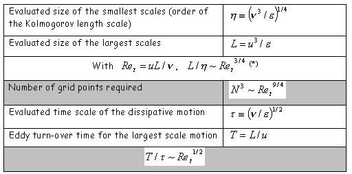
(*) See Section 6

Thus, with time space consideration, a computation would have to be performed for systems requiring
Re^11/4 calculation points. In the mid-90’s, the maximum resolution attained in three dimensions was of the order of
300³ on a CRAY 2 machine. With Reynolds numbers typically encountered in industrial systems (above
10⁴ order of magnitude), the required number of spatial grid points and resultant time steps are far beyond the capacity of present day computers. DNS is therefore expected to remain limited to academic applications (on turbulence research …) still for a distant future, despite the advance of parallel computing techniques which are only at the preliminary stage of their development when applied to fluid dynamics.

This procedure is discussed further in

CF37

Generally, engineers are more interested in the description of the large scales of the flow, which often contain the desired information about turbulent transfers of momentum or heat. It is these large scales, which ought to be simulated. Thus, there are essentially two other alternative routes for their prediction – LES and Turbulence Modelling approach.

4. LES

The [GLOSS]LES[/GLOSS] – procedure involves the solution of the 3D time-dependent Navier-Stokes equations and the direct simulation of the large scales motion. This approach requires the representation (model) of the energy exchanges with the small scales, which are not explicitly simulated, complicated by the molecular diffusion scales phenomena encountered in combusting or reacting flows leading to the use of a sub-grid model for the statistics of the small scale motion.

As LES simulations provide time-dependent results, they prove helpful to pinpoint flow instabilities, not obtainable from standard methods based on Navier-Stokes’ equation averaging. Industry starts implementing LES techniques as complement to more classical approaches.

This procedure is discussed further in

CF36

5. Turbulence modelling approach

Looking at a typical point velocity measurement in a turbulent flow shows that the instantaneous velocity can be decomposed into a steady mean value U with a superimposed fluctuating component u’(t). A similar derivation can be applied to any flow property
(j).

Averaging the Navier-Stokes equations over a time, dt, long compared to that of the turbulent motion (conventional time-averaging for steady state formulation can be used in the majority of cases) yields the equation of the
mean motion. This statistical process introduces in the mean momentum equations unknown turbulent correlations, the
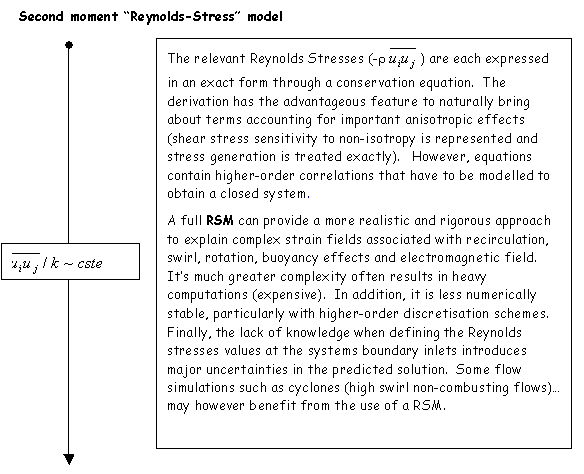
Reynolds Stresses, which represent the transport of momentum due to turbulence. In order to close these transport equations, a
turbulence model must be introduced to determine the unknown turbulent [GLOSS]Reynolds Stresses[/GLOSS]. The choice of the set of turbulence equation(s) and the provision of closure approximations, in addition to the mean flow equations, constitute the
TURBULENCE MODELLING APPROACH (See definitions in Section 6.

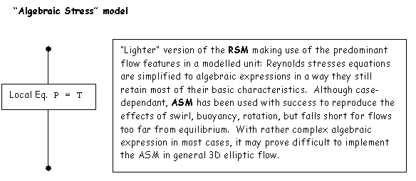
Models can be classified generally as Eddy-viscosity or Reynolds Stress Models and can be broadly cast within the following hierarchy (Note that in the following text images we introduce the acronyms [GLOSS]RSM[/GLOSS], [GLOSS]ASM[/GLOSS] and [GLOSS]RNG[/GLOSS]):

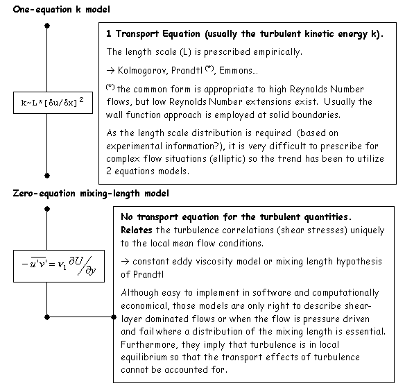
For no or low Swirl Number, high Reynolds Number combusting flows within industrial applications, the
k-e model (or derivations) represents a good compromise in terms of predictive outcome and computation economy.

As a general conclusion of this Combustion File, which only attempts to present the “tip of the turbulence modelling iceberg”, related topics must be pointed out: Use of “wall-functions” on solid surface boundaries; Low Reynolds Number adaptations of turbulence models; Multi-scale
k-e models; Two_layer
k-e model; Multi-fluid turbulence models; Renormalising Group Theory (RNG) or Renormalising Perturbation Theory for turbulence modelling (form comparable to a LES procedure); Particles_turbulence interactions/modulations in multiphase
flows. These will be explored in due course.

6. Terminology Clarifications

Eddy viscosity hypothesis: By analogy with molecular viscosity, which is a fluid property, turbulence is often described using the concept of eddy viscosity as a local property of the fluid, the corresponding mixing length being treated in an analogous manner to the molecular mean-free path derived from the kinetic theory of gases. This description is based on erroneous physical concepts but has proved useful in the quantitative prediction of simple turbulence flows.

Turbulent (or eddy) kinematic viscosity – – is not a fluid property but depends on the local state of turbulence. It is assumed to be a scalar of dimension
m²/s and vary significantly from point to point and flow to flow. It can be easily defined as the product of a turbulent velocity scale
x
(m/s – “resembling the velocity fluctuations”) and an integral length scale L (m). Dimensional analysis yields
. 

Consequently, the averaged Navier-Stokes equations are expressed with the
term effective dynamic viscosity
m_eff
= m
+
m_t
, where m
represents the molecular dynamic viscosity.

The kinetic energy of a turbulent motion (k) is a measure of normal (or diagonal) turbulence stresses:

The turbulent Reynolds Number is obtained from the flow Reynolds Number when the turbulent kinetic energy
(k) and the integral length scale (L) are substituted in place of the mean flow velocity and system characteristic dimension respectively: 

Re_t is an attempt to achieve a better description of the degree of turbulence: it is a measure of the ratio between integral length scale (L) and Kolmogorov length scale
(h):
.

Acknowledgements

Special thanks to Jacques Dugué and all my colleagues at CINAR for their skilled and valuable comments.